Tutorial 4: Two-Dimensional Conversion Functions

pygid supports several representations of 2D conversion: GID, Cartesian, polar, and pseudopolar.

Table 1. Conversion functions with description

Function	Description	Name of Output Image	Corresponding Matrix Coordinates
det2q_gid()	GID coordinates	img_gid_q	q_xy, q_z
det2pol_gid()	Polar coordinates for GID experiments	img_gid_pol	q_gid_pol, ang_gid_pol
det2pseudopol_gid()	Pseudopolar coordinates for GID experiments	img_gid_pseudopol	q_gid_azimuth, q_gid_rad
det2q()	Cartesian coordinates for transmission experiments	img_q	q_x, q_y
det2pol()	Polar coordinates for transmission experiments	img_pol	q_pol, ang_pol
det2pseudopol()	Pseudopolar coordinates for transmission experiments	img_pseudopol	q_azimuth, q_rad

Note: In this tutorial, only GID and polar conversions are described. All other conversion functions (det2pseudopol_gid(), det2q(), det2pol(), det2pseudopol()) use the same parameters and workflow.

Load datasets from Zenodo, and create params, matrix, and analysis instances as described in Tutorials 1–3.

from shapely.speedups import available

from pygid.datasets import get_dataset

# Download example dataset from Zenodo
try:
    files = get_dataset("tutorial_04")
    poni_path = files["poni"]
    mask_path = files["mask"]
    # several files for batch processing
    data_path = files["data"]
except:
    print("Dataset download skipped on Read the Docs.")

---------------------------------------------------------------------------
ModuleNotFoundError                       Traceback (most recent call last)
Cell In[1], line 1
----> 1 from shapely.speedups import available
      2 
      3 from pygid.datasets import get_dataset
      4 

ModuleNotFoundError: No module named 'shapely'

import pygid

# create pygid.ExpParams based on the PONI file
params = pygid.ExpParams(
    poni_path=poni_path,          # path to the PONI file
    mask_path=mask_path,
    ai=0.01,                       # angle of incidence (degrees)
    fliplr=True,
    flipud=True
)

# create pygid.CoordMaps based on pygid.ExpParams
matrix = pygid.CoordMaps(
    params  # pygid.ExpParams
)

# load the data from file
analysis = pygid.Conversion(
    matrix=matrix,                   # pygid.CoordMaps
    path=data_path,                  # path to the raw data file
    dataset='/entry_0000/ESRF-ID10/eiger4m/data'  # dataset path
)
print(f"raw data shape {analysis.img_raw.shape}")

raw data shape (13, 2162, 2068)

---

Minimal Code Example

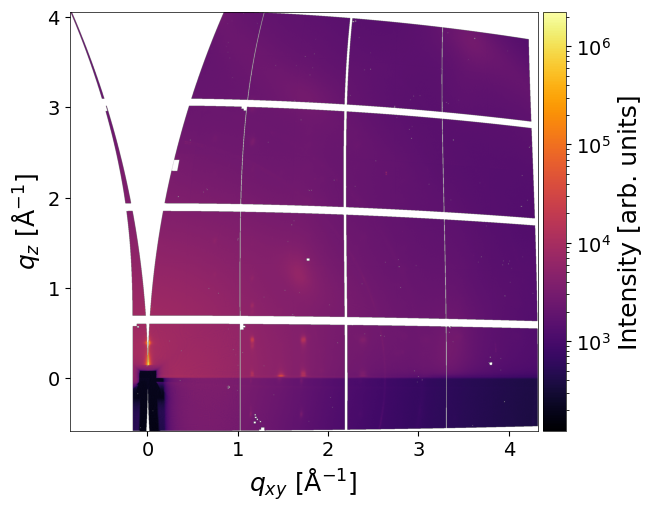
analysis.det2q_gid(
    frame_num=7,                   # frames to convert; None = all images
    plot_result=True
)

---

Parameters (for all remapping functions)

Main parameters:

• frame_num – index or list of indiced of loaded frames to convert (not the frame number in file). If None, all loaded images are converted.

• return_result – if True, returns converted image and axes arrays. Default is False.

• interp_type – interpolation method for remapping ("INTER_LINEAR", "INTER_NEAREST", etc.). Default: "INTER_LINEAR".

• multiprocessing – flag to enable multiprocessing. If None, uses the default defined in the Conversion class.

• q_xy_range - q_xy range (tuple, in Å⁻¹) for det2q_gid() function

• q_z_range - q_z range (tuple, in Å⁻¹) for det2q_gid() function

• radial_range - radial range range (tuple, in Å⁻¹) for det2pol_gid() function

• angular_range - angular range range (tuple, in degrees) for det2pol_gid() function

Saving parameters:

• save_result – whether to save the result as an HDF5 file in NXsas format.

• path_to_save – output path for the HDF5 result file.

• h5_group – name of the NXentry dataset within the HDF5 file.

• overwrite_file – if True, overwrites existing HDF5 file. Default is True.

• overwrite_group – if True, overwrites existing NXentry group. Default is True.

• exp_metadata – ExpMetadata instance containing experimental information (see Tutorial 6).

• smpl_metadata – SampleMetadata instance containing sample information (see Tutorial 6).

Plotting parameters:

• plot_result – whether to plot the remapped image.

• clims – tuple (vmin, vmax) defining color scale limits.

• xlim, ylim – tuples defining X and Y axis limits for the plot.

• save_fig – whether to save the plotted image to a file.

• path_to_save_fig – path to save the plot (e.g. .png, .tiff).

Reciprocal Space Conversion (GID Geometry)

q_xy, q_z, img = analysis.det2q_gid(
    frame_num=[5,6,7],                   # frames to convert; None = all images
    plot_result=True,
    return_result=True,
    clims=(4e2,1e5),
    q_xy_range = (0,3.5),
    q_z_range = (0,3.5),
)

print(f"x-axis shape {q_xy.shape}")
print(f"y-axis shape {q_z.shape}")
print(f"length of images and their shape {len(img), img[0].shape}")

x-axis shape (1506,)
y-axis shape (1506,)
length of images and their shape (3, (1506, 1506))

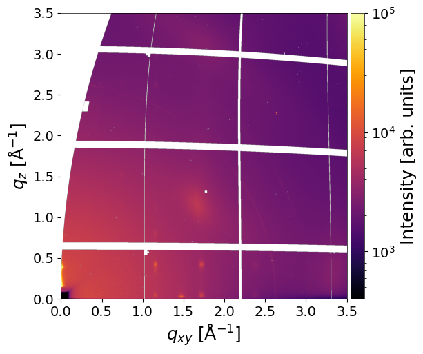
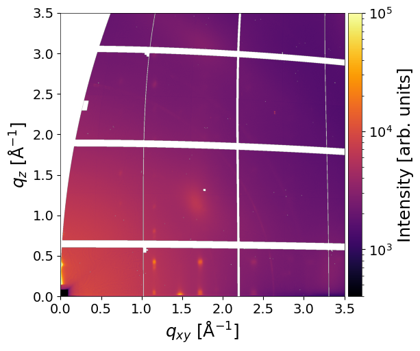
Polar Conversion (GID Geometry)

q_xy, q_z, img = analysis.det2pol_gid(
    frame_num=7,                   # frames to convert; None = all images
    plot_result=True,
    return_result=True,
    clims=(4e2,1e5),
    angular_range = (0,90)  #
)

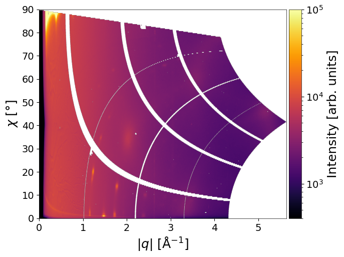
Accessing Converted Data

The results of a conversion can be retrieved using the pygid.Conversion.get_result() method after the conversion has been performed. The converted data are available only in memory and can be accessed before they are saved to disk.

analysis.det2pol_gid(
    plot_result=False,
)

x, y, img = analysis.get_result(
    frame_num=None,                        # frames to convert (int or list); None = all images
)

x.shape, y.shape, len(img), img[0].shape

((2428,), (1200,), 13, (1200, 2428))

Plotting After Conversion

The results of the conversion can be visualized immediately after processing by calling plot_result. The method optionally returns the numerical data arrays and supports plotting of selected frames.

x, y, img = analysis.plot_result(
    return_result=True,                 # return data arrays
    frame_num=0,                        # frames to plot (int or list); None = all images
    plot_result=True,                   # plot result
    clims=(4e2,1e5),                    # intensity limits
    save_fig=True,                      # save plot flag
    path_to_save_fig="graph.tiff",      # save plot path
)

NOTE: Plot parameters can be changed using pygid.set_plot_defaults function as shown in Tutorial 3

Saving of the Result

Converted data can be saved as an NXsas file (NeXus / HDF5) with a dedicated internal structure.

The output file can store:

• multiple images in a single entry, or

• images in different entries within the same file.

To save results from multiple pygid.Conversion instances into one file, set overwrite_file = False. In this case, all images must have the same shape (same q-range and resolution). If the shape differs, a new entry is created automatically.

The saved file also contains:

• PONI file information

• full details of the conversion parameters

For viewing and inspecting the resulting NeXus files, silx view is recommended.

Experimental and sample metadata can also be stored in the file; this is described in Tutorial 6.

q_xy, q_z, img = analysis.det2q_gid(
    frame_num=None,
    plot_result=False,
    return_result=True,
    clims=(4e2,1e5),
    q_xy_range=(0,3.5),
    q_z_range=(0,3.5),
    save_result=True,
    path_to_save='result.h5'
)

print(f"x-axis shape {q_xy.shape}")
print(f"y-axis shape {q_z.shape}")
print(f"length of images and their shape {len(img), img[0].shape}")

13 converted images have been saved in ‘result.h5’ as a single dataset

Modifying and Saving Data After Conversion

Converted data can be modified in memory after the conversion step and before saving. This allows for post-processing adjustments prior to writing the final HDF5 output.

# Run conversion without saving
analysis.det2q_gid(save_result=False)

# Modify converted image data
# (must remain a list of 2D NumPy arrays)
analysis.img_gid_q[0] /= 2

# Save results to HDF5
pygid.DataSaver(
    analysis,                    # pygid.Conversion instance
    path_to_save='result.h5',    # path to save
    overwrite_file=True,         # Whether to overwrite an existing HDF5 file
    overwrite_group = True,      # Whether to overwrite an existing HDF5 entry
    h5_group = 'entry_0000',          # The specific group in the HDF5 file
)

NOTE: a new conversion overwrites the result of previous conversion in memory