Tutorial 9: GID pattern simulation

This tutorial uses the pygidSIM package to simulate GIWAXS patterns based on a CIF file describing the crystal structure. The function make_simulation() overlays simulated diffraction peaks onto the experimental GIWAXS image.

Before starting, download the required datasets from Zenodo (or provide your own data files) and create an analysis instance as described in Tutorial 3.

from pygid.datasets import get_dataset

# Download example dataset from Zenodo
try:
    files = get_dataset("tutorial_09")
    data_path = files["data_peaks"]
    poni_path = files["poni_peaks"]
    mask_path = files["mask_peaks"]
    cif_path_peaks = files["cif_peaks"]
except:
    print("Dataset download skipped on Read the Docs.")

Dataset download skipped on Read the Docs.

import pygid

# create pygid.ExpParams based on the PONI file
params = pygid.ExpParams(
    poni_path=poni_path,          # path to the PONI file
    mask_path=mask_path,
    ai=0.01,                       # angle of incidence (degrees)
    fliplr=True,
    flipud=True
)

# create pygid.CoordMaps based on pygid.ExpParams
matrix = pygid.CoordMaps(
    params,  # pygid.ExpParams
    hor_positive=True,
    vert_positive=True
)

# load the data from file
analysis = pygid.Conversion(
    matrix=matrix,                   # pygid.CoordMaps
    path=data_path,                  # path to the raw data file
    dataset='/entry_0000/ESRF-ID10/eiger4m/data',  # dataset path
    frame_num=7
)

Parameters

• frame_num : int Frame index of the experimental data to plot.

• crystal : dict or list of dict Crystal description(s). Each dictionary should contain:

  • 'path_to_cif' : str — path to the .cif file, or alternative crystal definition.

  • 'orientation' : array-like [u, v, w] or str "random" — orientation of the crystal in the laboratory frame.

  • 'min_int' : float — minimum normalized intensity to include in the simulation/plot.

  A list of dictionaries can be provided to simulate multiple crystals in one call.

---

Minimal code example

crystal = {
    'path_to_cif': cif_path_peaks,
    'orientation': [0,0,1],
    'min_int': 1e-3,
}

analysis.make_simulation(
    frame_num=0,                  # Frame of experimental data
    crystal=crystal,
    plot_result=True,             # Display simulation overlay
    clims=(4e2,1e5),              # Intensity limits
)

INFO - Simulating GIWAXS data from CIF: /home/ainurabukaev/.cache/pygid/tutorial_09/DIP_thin_film_642482.cif, orientation: [0, 0, 1]

---

Crystal Description Dictionary

crystal is a dictionary that defines a single crystal for simulation and plotting in GIWAXS workflows. Each key controls either the crystal structure, orientation, intensity filtering, or optional plotting parameters.

Keys Description:

• `path_to_cif (str): Path to the CIF file containing the crystal structure.

• orientation (array-like [u, v, w] or str “random”): Crystal orientation (contact plane) in the laboratory frame.

• min_int (float): Minimum normalized intensity to include in the simulation/plot.

Optional Plotting Parameters:

• cmap (str): Colormap for intensity visualization.

• vmin, vmax (float): Colormap normalization limits.

• marker (str), marker_size (float): Style and size of plotted peaks.

• line_width (float), line_style (str): Line style for rings.

• plot_mi (bool): Whether to overlay Miller indices.

• text_color (str): Color of Miller indices.

• text_size (int): Size of Miller indices.

Other parameters

• return_result – if True, returns a simulation result object.

• save_fig – if True, saves the resulting image.

• path_to_save_fig – filename for saving the image.

• move_fromMW – if True, moves reflections from the missing wedge to the border.

• clims, xlim, ylim - Color and axes limits for the figure.

---

Single simulation example

Oriented crystal

crystal_1 = {
    'path_to_cif': cif_path_peaks,
    'orientation': [0,0,1],  # 3x1 vector [u, v, w] or "random"
    'min_int': 1e-3,         # Minimum normalized intensity to include
    'cmap': 'winter',
    'plot_mi': False,
    'vmin': 0.01,
    'vmax': 1,
    'marker': 'o',
    'marker_size': 50,
    'line_width': 1,
    'line_style': "dashed",
    'text_color': "black"
}

q_values, intensity, mi = analysis.make_simulation(
    frame_num=0,                  # Frame of experimental data
    crystal = crystal_1,
    clims=(4e2,1e5),              # Color scale limits for experimental image
    plot_result=True,             # Display simulation overlay
    plot_mi=False,                # Annotate peaks with Miller indices
    return_result=True,           # Return simulation result
)

INFO - Simulating GIWAXS data from CIF: /home/ainurabukaev/.cache/pygid/tutorial_09/DIP_thin_film_642482.cif, orientation: [0, 0, 1]

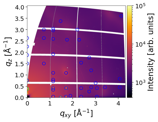
The simulated peaks are visualized as circles, with colors proportional to their intensity. The color scale can be controlled using the vmin and vmax parameters, and the size of the circles can be adjusted with the radius parameter. When return_result=True, the function returns:

• q_values – a 2D array of peak positions (q_xy, q_z) (in Å⁻¹)

• intensity – array of simulated peak intensities

• mi – corresponding Miller indices for each peak

# results shape
q_values.shape, intensity.shape, mi.shape

((2, 42), (42,), (42, 3))

# split the q_values
q_xy = q_values[0]
q_z = q_values[1]

Peaks located in the missing wedge can be moved to the border by setting the move_fromMW=True flag:

q_values, intensity, mi = analysis.make_simulation(
    frame_num=0,                  # Frame of experimental data
    crystal = crystal,
    clims=(4e2,1e5),              # Color scale limits for experimental image
    plot_result=True,             # Display simulation overlay
    plot_mi=False,                # Annotate peaks with Miller indices
    return_result=True,           # Return simulation result
    move_fromMW=True
)

INFO - Simulating GIWAXS data from CIF: /home/ainurabukaev/.cache/pygid/tutorial_09/DIP_thin_film_642482.cif, orientation: [0 0 1]

Random orientation

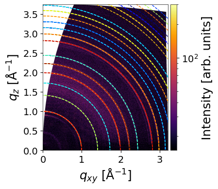
The make_simulation() function can also simulate and plot diffraction rings for randomly oriented crystals. To enable this, set orientation to "random". The sharpness of the plotted rings can be controlled using the linewidth parameter.

When return_result=True, the function returns:

• q_values – a 1D array of absolute q-values (q_abs) (in Å⁻¹)

• intensity – array of simulated peak intensities

• mi – corresponding Miller indices for each peak

from pygid.datasets import get_dataset

# Download example dataset from Zenodo
try:
    files = get_dataset("tutorial_09")
    data_path = files["data_rings"]
    poni_path = files["poni_rings"]
    cif_path_rings = files["cif_rings"]
except:
    print("Dataset download skipped on Read the Docs.")

import pygid

# create pygid.ExpParams based on the PONI file
params = pygid.ExpParams(
    poni_path=poni_path,          # path to the PONI file
    ai=0.01,                       # angle of incidence (degrees)
    fliplr=False,
    flipud=True
)

# create pygid.CoordMaps based on pygid.ExpParams
matrix = pygid.CoordMaps(
    params,  # pygid.ExpParams
    hor_positive=True,
    vert_positive=True
)

# load the data from file
analysis = pygid.Conversion(
    matrix=matrix,                   # pygid.CoordMaps
    path=data_path,                  # path to the raw data file
)

crystal_2 = {
    'path_to_cif': cif_path_rings,
    'orientation': "random",  # 3x1 vector [u, v, w] or "random"
    'min_int': 1e-5,         # Minimum normalized intensity to include
    'cmap': 'jet',
    'plot_mi': False,
    'vmin': 0.01,
    'vmax': 1,
    'line_width': 1,
    'line_style': "dashed",
    'text_color': "black"
}

q_values, intensity, mi = analysis.make_simulation(
    frame_num=0,                  # Frame of experimental data
    crystal = crystal_2,
    clims=(15,300),              # Color scale limits for experimental image
    plot_result=True,             # Display simulation overlay
    plot_mi=False,                # Annotate peaks with Miller indices
    return_result=True,           # Return simulation result
    move_fromMW=True
)

INFO - Simulating GIWAXS data from CIF: /home/ainurabukaev/.cache/pygid/tutorial_09/MAPBTI02 - stoumpos_cubicMAPbI3.cif, orientation: random

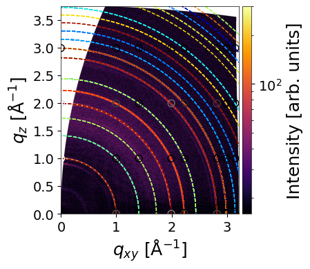
The rings and arcs observed at 0.45, 0.51, and 0.65 Å⁻¹ are not simulated, as they originate from a Pb₃I₈ intermediate complex.

Crystal description

To calculate a GIWAXS pattern from the own description instead of the CIF file, use the following example from pygidSIM description:

import numpy as np

# space group number
spgr = 221  # alternatively, use e.g. '146:R'

# lattice parameters [a, b, c, α, β, γ]
lat_par = np.array([6.3026, 6.3026, 6.3026, 90., 90., 90.], dtype=np.float32)

# list of atoms
atoms = np.array(['Pb', 'I', 'I', 'I', 'N'])

# relative atom positions
atom_positions = np.array(
    [[0., 0., 0.],
     [0.5, 0., 0.],
     [0., 0.5, 0.],
     [0., 0., 0.5],
     [0.5, 0.5, 0.5]], dtype=np.float32
)

# occupancies of the corresponding sites
occupancy = np.array([1., 1., 1., 1., 1.], dtype=np.float32)

crystal_3 = {
    'spgr': 221,
    'lat_par': lat_par,
    'atoms': atoms,
    'atom_positions': atom_positions,
    'occupancy': occupancy,
    'orientation': [0,0,1],
    'min_int': 0.002,
    'cmap': 'gray',
    'plot_mi': False,
    'vmin': 0.1,
    'vmax': 1,
    'marker': 'o',
    'marker_size': 50,
    'line_width': 1,
    'line_style': "dashed",
    'text_color': "black"
}

Multiple Simulations

To plot multiple simulated patterns from different crystal or orientations, make_simulation() accepts lists for the dictionaries as crystal parameter:

When return_result=True, the function returns list of tuple for each crystal:

result_list = analysis.make_simulation(
    frame_num=0,
    clims=(16,300),
    crystal=[crystal_2, crystal_3],         # List of CIFs
    plot_result=True,
    plot_mi=False,
    return_result=True,
)

INFO - Simulating GIWAXS data from CIF: /home/ainurabukaev/.cache/pygid/tutorial_09/MAPBTI02 - stoumpos_cubicMAPbI3.cif, orientation: random
INFO - Simulating GIWAXS data from Crystal, orientation: [0, 0, 1]
INFO - Use already converted image with frame num 0

result_list is a list of tuples: q_values, intensity, mi:

len(result_list)

2