Tutorial 10. Transmission Geometry and GISAXS

Transmission Geometry

Although the pygid package was originally developed for GIWAXS data, it can also be applied to transmission experiments using the same functionality. All features described in Tutorials 1–6 and 8 are available for this type of measurement.

For transmission experiments, the angle of incidence ai should be set to 0°, and functions should use the names without the _gid suffix.

The following table summarizes the available two-dimensional conversions and line profile functions:

Function Name	Output Data Name	Axes Name	Description
det2q()	img_q	q_x, q_y	Converts detector coordinates to Cartesian q-space for transmission experiments
det2pol()	img_pol	q_pol, ang_pol	Converts to polar coordinates for transmission experiments
det2pseudopol()	img_pseudopol	q_azimuth, q_rad	Converts to pseudopolar coordinates for transmission experiments
radial_profile()	rad_cut	q_pol	Computes polar remapping and averages intensity within a specified angular range (transmission geometry)
azim_profile()	azim_cut	ang_pol	Computes polar remapping and averages intensity within a specified radial range (transmission geometry)

The full list of parameters is described in Tutorials 1–6 and 8; here we provide only short usage examples.

First, load the transmission data:

from pygid.datasets import get_dataset

# Download example dataset from Zenodo
try:
    files = get_dataset("tutorial_10")
    data_path = files["data"]
    poni_path = files["poni"]
except:
    print("Dataset download skipped on Read the Docs.")

Create the pygid.Conversion instance:

import pygid

# create pygid.ExpParams based on the PONI file
params = pygid.ExpParams(
    poni_path=poni_path,          # path to the PONI file
    ai=0,                         # angle of incidence 0 for the transmission geometry
    fliplr=False,
    flipud=True
)

# create pygid.CoordMaps based on pygid.ExpParams
matrix = pygid.CoordMaps(
    params,  # pygid.ExpParams
    hor_positive=True,
    vert_positive=True
)

# load the data from file
analysis = pygid.Conversion(
    matrix=matrix,                   # pygid.CoordMaps
    path=data_path,                  # path to the raw data file
)

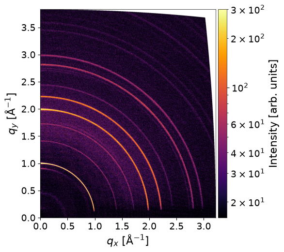
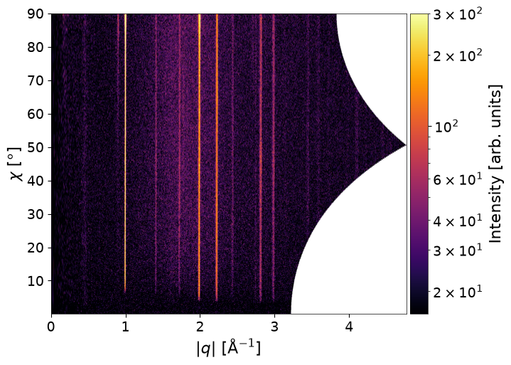
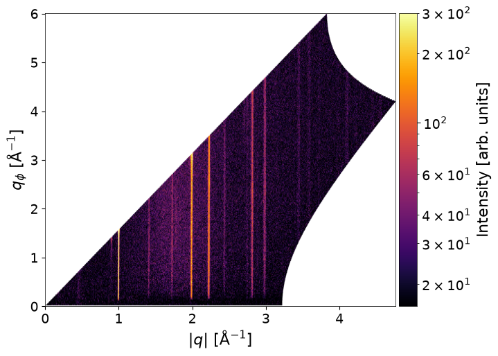
Two-dimensional conversion

q_x, q_y, img =  analysis.det2q(plot_result=True, return_result=True, clims=(16,300))
q_abs, ang, img = analysis.det2pol( plot_result=True, return_result=True, clims=(16,300))
q_rad, q_azim, img = analysis.det2pseudopol(plot_result=True, return_result=True, clims=(16,300))

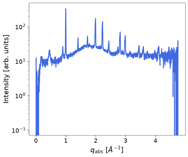
One-dimensional conversion

q_abs, img =  analysis.radial_profile(plot_result=True, return_result=True)
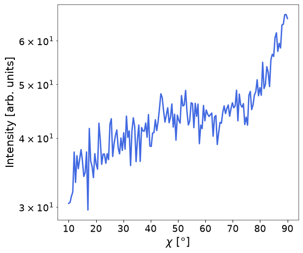
chi, img = analysis.azim_profile( plot_result=True, return_result=True,
                                  radial_range = (1.9, 2.1), # radial range in A-1
                                  angular_range = (10, 90)   # angular range in A-1
                                  )

GISAXS

For many practical cases, the effect of the missing wedge at very small exit angles can be neglected, allowing the use of transmission-geometry functions for approximate analysis. However, for quantitative studies near the critical angle or for very thin films, missing-wedge corrections may be necessary.